Dictionary
Statistics, Information Theory and ML
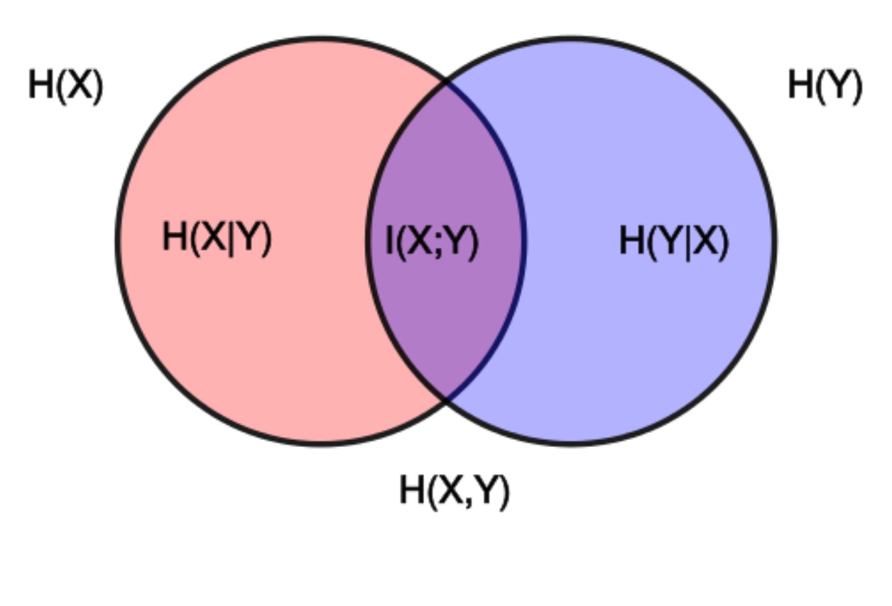
Entropy, conditional entropy, and mutual information
\[ {\displaystyle {\begin{aligned}\operatorname {I} (X;Y)&{}\equiv \mathrm {H} (X)-\mathrm {H} (X\mid Y)\\&{}\equiv \mathrm {H} (Y)-\mathrm {H} (Y\mid X)\\&{}\equiv \mathrm {H} (X)+\mathrm {H} (Y)-\mathrm {H} (X,Y)\\&{}\equiv \mathrm {H} (X,Y)-\mathrm {H} (X\mid Y)-\mathrm {H} (Y\mid X)\end{aligned}}} \]
 |
Expected score in MLE is zero
\(f(z;\theta)\) is the density function, for data \(z\), and parameter vector \(\theta\), so \(\int f(z;\theta)dz=1\) for any \(\theta\).
\[ \int \frac{\partial f(z;\theta)}{\partial \theta}dz=0 \Leftrightarrow \int \frac{f(z;\theta)}{f(z;\theta)} \frac{\partial f(z;\theta)}{\partial \theta}dz=0\Leftrightarrow \int f(z;\theta) \frac{\partial log f(z;\theta)}{\partial \theta}dz=0 \]
Fisher information
The Fisher information is defined to be the variance of the score:
\[ \mathcal{I}(\theta) = \operatorname{E} \left[\left. \left(\frac{\partial}{\partial\theta} \log f(X;\theta)\right)^2\right|\theta \right] = \int_{\mathbb{R}} \left(\frac{\partial}{\partial\theta} \log f(x;\theta)\right)^2 f(x; \theta)\,dx = - \operatorname{E} \left[\left. \frac{\partial^2}{\partial\theta^2} \log f(X;\theta)\right|\theta \right], \]
The Fisher information may be seen as the curvature of the support curve (the graph of the log-likelihood). Near the maximum likelihood estimate, low Fisher information therefore indicates that the maximum appears “blunt”, that is, the maximum is shallow and there are many nearby values with a similar log-likelihood. Conversely, high Fisher information indicates that the maximum is sharp.
Relation of Fisher information to relative entropy
Fisher information is related to relative entropy. The KL-divergence between two distributions in the family can be written as
\[ D(\theta,\theta’) = KL(p({}\cdot{};\theta):p({}\cdot{};\theta’))= \int f(x; \theta)\log\frac{f(x;\theta)}{f(x; \theta’)} \, dx. \]
If \({\displaystyle \theta }\) is fixed, then the relative entropy between two distributions of the same family is minimized at \({\displaystyle \theta ’=\theta }\). For \({\displaystyle \theta ’}\) close to \({\displaystyle \theta }\), one may expand the previous expression in a series up to second order:
\[ D(\theta,\theta’) = \frac{1}{2}(\theta’ - \theta)^\textsf{T} \left(\frac{\partial^2}{\partial\theta’_i\, \partial\theta’_j} D(\theta,\theta’)\right)_{\theta’=\theta}(\theta’ - \theta) + o\left( (\theta’-\theta)^2 \right) \]
But the second order derivative can be written as
\[ \left(\frac{\partial^2}{\partial\theta’_i\, \partial\theta’_j} D(\theta,\theta’)\right)_{\theta’=\theta} = - \int f(x; \theta) \left( \frac{\partial^2}{\partial\theta’_i\, \partial\theta’_j} \log(f(x; \theta’))\right)_{\theta’=\theta} \, dx = [\mathcal{I}(\theta)]_{i,j} \]
Thus the Fisher information represents the curvature of the relative entropy of a conditional distribution with respect to its parameters.
Entropy, cross entropy and KL divergence
Assume two distributions \(p\) and \(q\)
Entropy of \(p\) is
\[ H(p)=-E_{p}[\log p]=-\int p(y)\log p(y)dy \]
The cross-entropy of the distribution \(q\) relative to a distribution \(p\) is
\[ H(p,q)=-E_{p}[\log q]=-\int p(y)\log q(y)dy \]
The KL divergence (the relative entropy from \(q\) to \(p\) is
\[ D_{\mathrm{KL}}(p\|q)=-\int p(y)\log\frac{q(y)}{p(x)}dy \]
We have the relationship
\[ H(p,q)=H(p)+D_{\mathrm{KL}}(p\|q) \]
Logistic regression
The predicted probability of the output
\[ h_{w}(x)={\displaystyle \widehat{P}(y=1|x)\equiv{\frac{1}{1+e^{-w^{\top}x}}}} \]
\[ {\displaystyle 1-h_{w}(x)}=1-\widehat{P}(y=1|x)=\widehat{P}(y=0|x) \]
The logistic loss is
\[ L(y,h_{w})=\begin{cases} -\log(h_{w}) & \text{if }y=1\\ -\log(1-h_{w}) & \text{if }y=0 \end{cases} \]
which is the negative log probability that \(y\) is classified as its correct class. Since \(y\in\{0,1\}\)
\[ L(y,h_{w}(x))=-y\log(h_{w}(x))-(1-y)\log(1-h_{w}(x)) \]
Sum over \(n\) samples
\[ L(w)=\sum_{i=1}^{n}\left[-y_{i}\log(h_{w}(x_{i}))-(1-y_{i})\log(1-h_{w}(x_{i}))\right] \]
Analysis
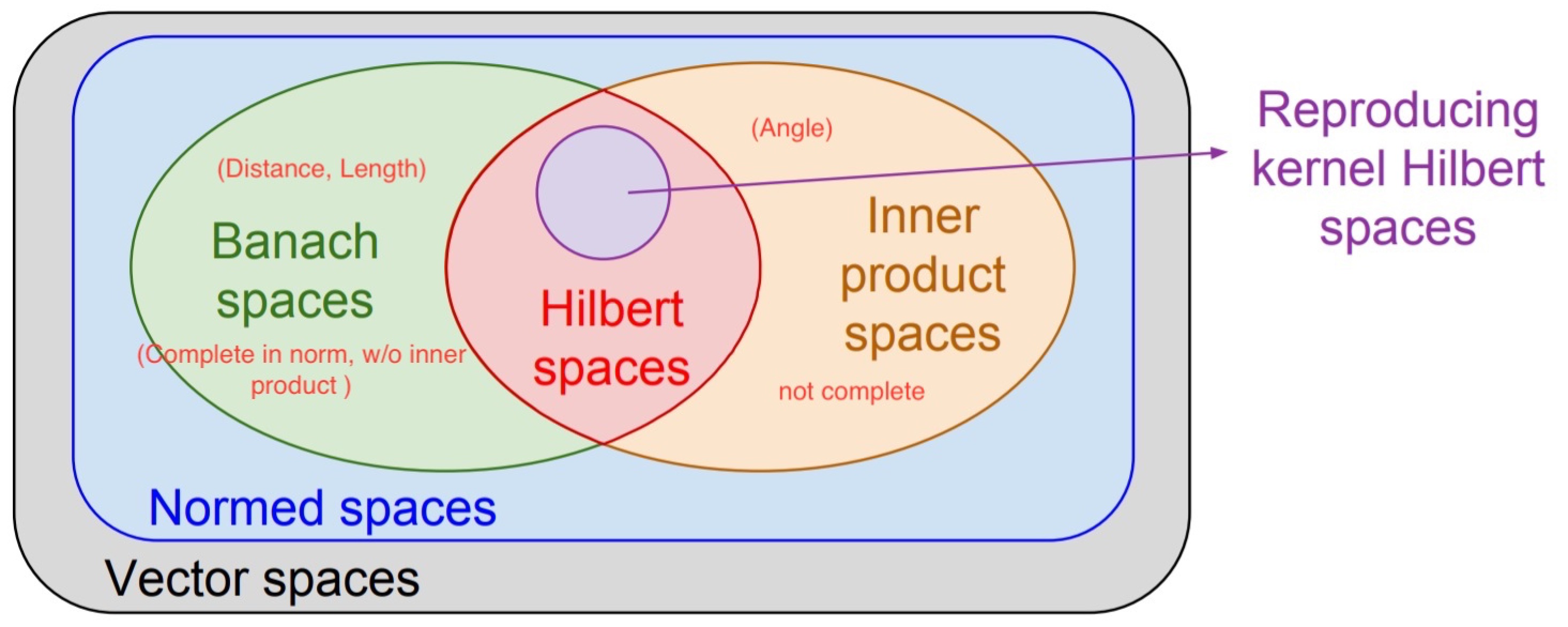
Hilbert space
Euclidean space \(\subset\) Hilbert space \(\subset\) Banach \(\subset\) Metric space
 |
log-sum-exponential
The log-sum-exponential (LSE) function is commonly used as a smooth approximation of the maximum function. The LSE function is defined as:
\[ \text{LSE}(x_1, x_2, \dots, x_n) = \log\left( \sum_{i=1}^n e^{x_i} \right) \]
This function has properties that make it a smooth and differentiable approximation of the maximum of the inputs \(x_i\). Specifically, as the inputs become larger, the exponentials of the smaller \(x_i\) become negligible compared to the exponential of the maximum \(x_{\text{max}}\) , and the LSE converges to \(x_{\text{max}}\):
\[ \lim_{k \to \infty} \frac{1}{k} \log\left( \sum_{i=1}^n e^{k x_i} \right) = \max(x_1, x_2, \dots, x_n) \]
This property is particularly useful in optimization and machine learning because it allows for gradient-based optimization methods. The LSE function is convex and differentiable everywhere, which facilitates the computation of gradients.
Example: Suppose you have two numbers, \( x \) and \( y \). The maximum function is not differentiable at points where \( x = y \), but the LSE function provides a smooth approximation:
\[ \text{LSE}(x, y) = \log\left( e^x + e^y \right) \]
This function is smooth and has continuous derivatives with respect to \(x\) and \(y\).
Connection between log-sum-exponential and softmax
Consider the LSE function:
\[ f(x) = \log\left( \sum_{i=1}^{n} e^{x_i} \right) \]
The partial derivative with respect to \(x_k\) is:
\[ \frac{\partial f}{\partial x_k} = \frac{e^{x_k}}{\sum_{j=1}^{n} e^{x_j}} = \text{Softmax}(x_k) \]
This shows that the softmax function emerges naturally as the gradient of the LSE function.
Computing the softmax function directly can lead to numerical instability due to large exponentials. By leveraging the LSE function, we can rewrite the softmax function to improve numerical stability:
\[ \text{Softmax}(x_i) = e^{x_i - \text{LSE}(x_1, x_2, \dots, x_n)} \]
Stirling's approximation
More precise formula
\[ n! \sim \sqrt{2 \pi n}\left(\frac{n}{e}\right)^n \]
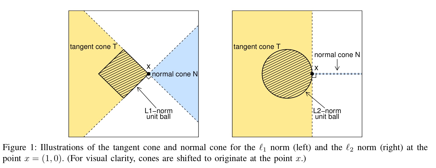
Tangent cone
Define the tangent cone of a convex set \(\mathcal{C}\) at a point \(z\) to be the set
\[ \mathcal{K}_{\mathcal{C}}(z) = \{ \Delta \in \mathbb{R}^n: \Delta = t(x - z), \; \text{for some } t \geq 0, x \in \mathcal{C} \} \]
For example, If the set is
\[ \mathcal{C} = \{ \thet\overline{{A}^{\top}} \in \mathbb{R}^n : \| \thet\overline{{A}^{\top}} \|_1 \leq 1 \} \]
 |
|
Let \(K\) be a closed convex subset of a real vector space \(V\) and \(\partial K\) be the boundary of \(K\). The solid tangent cone to \(K\) at a point \(x \in \partial K\) is the closure of the cone formed by all half-lines (or rays) emanating from \(x\) and intersecting \(K\) in at least one point \(y\) distinct from \(x\). It is a convex cone in \(V\) and can also be defined as the intersection of the closed half-spaces of \(V\) containing \(K\) and bounded by the supporting hyperplanes of \(K\) at \(x\).
Sum of the supremum
See that \(f(\theta) \le \sup_{\Theta}f(\theta)\) and \(g(\theta) \le \sup_{\Theta}g(\theta)\) for all \(\theta \in \Theta\)
\[ f(\theta)+g(\theta) \le \sup_{\Theta} \left ( f(\theta)+g(\theta) \right ) \le \sup_{\Theta}f(\theta)+\sup_{\Theta}g(\theta) \]
Algebra
Holder's inequality
\[ \|fg\|_1 \le \|f\|_p \|g\|_q \]
Special case,
\[ \|fg\|_1 \le \|f\|_2 \|g\|_2 \]
Triangular inequality
The sum of the lengths of any two sides must be greater than or equal to the length of the remaining side.
\[ \|x\|+\|y\| \geq \|x+y\| \]
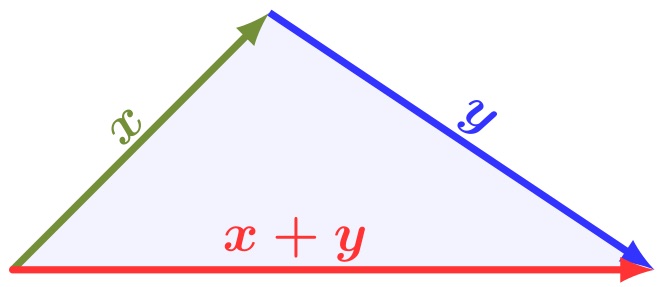 |
(from Wikipedia) |
Reverse triangle inequality
Any side of a triangle is greater than the difference between the other two sides.
\[ \bigg|\|x\|-\|y\|\bigg| \leq \|x-y\| \]
The proof for the reverse triangle uses the regular triangle inequality,
\[ \|x\| = \|(x-y) + y\| \leq \|x-y\| + \|y\| \Rightarrow \|x\| - \|y\| \leq \|x-y\| \]
\[ \|y\| = \|(y-x) + x\| \leq \|y-x\| + \|x\| \Rightarrow \|x\| - \|y\| \geq -\|x-y\| \]
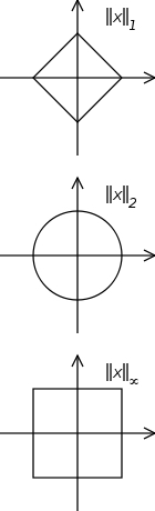
Vector norm inequality
\[ \left\| x \right\|_\infty \le \left\| x \right\|_2 \le \left\| x \right\|_1 \le \sqrt{n} \left\| x \right\|_2 \le n \left\| x \right \|_\infty \]
 |
Frobenius inner product
The Frobenius inner product is defined as,
\[ \langle {A}, {B} \rangle_\mathrm{F} =\sum_{i,j}\overline{A_{ij}} B_{ij} \, = \mathrm{Tr}\left(\overline{{A}^{\top}} {B}\right) = \mathrm{Tr}\left((\overline{A})^{\top} {B}\right) \]
When \(A\) is real
\[ \langle {A}, {B} \rangle_\mathrm{F} =\sum_{i,j}A_{ij} B_{ij} \, = \mathrm{Tr}\left({A}^{\top} {B}\right) \]
Also we have
\[ \|A\|^{2}_{F} = \langle {A}, {A} \rangle_\mathrm{F} = \mathrm{Tr}\left({A}^{\top} {A}\right) = \mathrm{Tr}\left({A} {A}^{\top}\right) \]
Trace
Trace of a product
If \(A\) and \(B\) are two \(m \times n\) real matrices
\[ \operatorname{tr}\left({A}^\mathsf{T}{B}\right) = \operatorname{tr}\left({A}{B}^\mathsf{T}\right) = \operatorname{tr}\left({B}^\mathsf{T}{A}\right) = \operatorname{tr}\left({B}{A}^\mathsf{T}\right) = \sum_{i=1}^m \sum_{j=1}^n a_{ij}b_{ij} \; . \]
Additionally, for real column vectors \({a}\in\mathbb{R}^n\) and \({b}\in\mathbb{R}^n\), the trace of the outer product is equivalent to the inner product:
\[ \operatorname{tr}\left({b}{a}^\textsf{T}\right) = {a}^\textsf{T}{b} \]
The symmetry of the Frobenius inner product may be phrased more directly as follows: the matrices in the trace of a product can be switched without changing the result. If \(A\) and \(B\) are \(m \times n\) and \(n \times m\) real or complex matrices, respectively, then
\[ \operatorname{tr}({A}{B}) = \operatorname{tr}({B}{A}) \]
Cyclic property
More generally, the trace is invariant under circular shifts, that is,
\[ \operatorname{tr}({A}{B}{C}{D}) = \operatorname{tr}({B}{C}{D}{A}) = \operatorname{tr}({C}{D}{A}{B}) = \operatorname{tr}({D}{A}{B}{C}). \]
Arbitrary permutations are not allowed: in general,
\[ \operatorname{tr}({A}{B}{C}) \ne \operatorname{tr}({A}{C}{B}). \]
However, if products of ’'three’’ symmetric matrix matrices are considered, any permutation is allowed, since:
\[ \operatorname{tr}({A}{B}{C}) = \operatorname{tr}\left(\left({A}{B}{C}\right)^{\mathsf T}\right) = \operatorname{tr}({C}{B}{A}) = \operatorname{tr}({A}{C}{B}), \]
where the first equality is because the traces of a matrix and its transpose are equal. Note that this is not true in general for more than three factors.
Trace as the sum of eigenvalues
Given any \(n \times n\) real or complex matrix \(A\), there is
\[ \operatorname{tr}({A}) = \sum_{i=1}^n \lambda_i \]
where \(\lambda_1,\ldots,\lambda_n\) are the eigenvalues of \(A\) counted with multiplicity. This holds true even if \(A\) is a real matrix and some (or all) of the eigenvalues are complex numbers.
Trace of the block matrix
For a block matrix \(A\)
\[ {A} = \begin{bmatrix} {A}_{11} & {A}_{12} & \cdots & {A}_{1q} \\ {A}_{21} & {A}_{22} & \cdots & {A}_{2q} \\ \vdots & \vdots & \ddots & \vdots \\ {A}_{q1} & {A}_{q2} & \cdots & {A}_{qq} \end{bmatrix} \]
We have
\[ \operatorname{tr}(A)=\operatorname{tr}(A_{11})+\operatorname{tr}(A_{22})+\cdots+\operatorname{tr}(A_{qq}) \]
Projection matrix
A square matrix \(P\) is called a projection matrix iff \(P^2 = P\).
A square matrix \(P\) is called an orthogonal projection matrix if \(P^2 = P = P^{\top}\) for a real matrix, and respectively \(P^2 = P = \overline{{P}^{\top}}\) for a complex matrix.
If \(P\) is a projection, so is \(I-P\).
Induced norm or operator norm
\[ \|A\| _p = \sup_{x \ne 0} \frac{\| A x\| _p}{\|x\|_p} \]
The induced operator norm shows by how much the “length” vector is stretched after applying the linear transformation \(A\), since
\[ \|Ax\|_{p} \leq \|A\|_{p}\|x\|_{p} \]
i.e. it satisfies the following property
\[ \|AB\|_p \leq \|A\|_p \|B\|_p \]
Since one can readily check
\[ \|Ax\|_{p}\leq\|A\|_{p}\|x\|_{p} \]
Apply this property twice, we get
\[ \|ABx\|_{p}\leq\|A\|_{p}\|Bx\|_{p}\leq\|A\|_{p}\|B\|_{p}\|x\|_{p} \]
Since this holds for any \(x\)
\[ \|AB\|_{p} = \sup_{x\neq 0} \frac{\|ABx\|_{p}}{\|x\|_{p}} \leq\|A\|_{p}\|B\|_{p} \]
In the special cases of \({\displaystyle p=1,2,\infty ,}\) the induced matrix norms can be computed or estimated by
Column sum norm
\(p=1\) Column sum
\[ \|A\|_1 = \max_{1 \leq j \leq n} \sum_{i=1}^m | a_{ij} | \]
Row sum norm
\(p=\infty\) Row sum norm
\[ \|A\|_\infty = \max_{1 \leq i \leq m} \sum _{j=1}^n | a_{ij} | \]
Spectral norm
\(p=2\) Spectral norm
\[ \|A\|_2 = \sqrt{\lambda_{\max}\left(\overline{{A}^{\top}} A\right)} = \sigma_{\max}(A) \]
“Entry-wise” matrix norms
These norms treat an \(m\times n\) matrix as a vector of size \(mn\), and use one of the familiar vector norms.
\[ \| A \|_{p,p} = \| \mathrm{vec}(A) \|_p = \left( \sum_{i=1}^m \sum_{j=1}^n |a_{ij}|^p \right)^{1/p} \]
Frobenius norm
The special case \(p = 2\) is the Frobenius norm,
\[ \| A \|_{2,2} = \| \mathrm{vec}(A) \|_2 = \left( \sum_{i=1}^m \sum_{j=1}^n |a_{ij}|^2 \right)^{1/2} = \|A\|_{F} \]
Max norm
The max norm is the elementwise norm in the limit as \(p \rightarrow \infty\) .
\[ \| A \|_{\infty,\infty} = \| \mathrm{vec}(A) \|_\infty = \left( \sum_{i=1}^m \sum_{j=1}^n |a_{ij}|^\infty \right)^{1/\infty} = \max_{ij} |a_{ij}| = \|A\|_{\max} \]
\[ \|AB\|_{\max} \nleq \|A\|_{\max} \|B\|_{\max} \]
\(L_{p,q}\) norm
For \(p,q\geq 1\), the \(L_{2,1}\) norm can be generalized to the \(L_{p,q}\) norm as follows:
\[ \| A \|_{p,q} = \left(\sum_{j=1}^n \left( \sum_{i=1}^m |a_{ij}|^p \right)^{\frac{q}{p}}\right)^{\frac{1}{q}} \]
Schatten norms
The Schatten \(p\)-norms arise when applying the \(p\)-norm to the vector of singular values of a matrix
\[ \|A\|^{\text{sh}}_p = \left( \sum_{i=1}^{\min\{m,n\}} \sigma_{i}^p(A) \right)^{\frac{1}{p}} \]
Trace (Nuclear) norm
\(p = 1\) Nuclear norm, Trace norm
\[ \|A\|^{\text{sh}}_1 = \|A\|_{*} = \operatorname{trace} \left(\sqrt{\overline{{A}^{\top}}A}\right) = \sum_{i=1}^{\min\{m,n\}} \sigma_{i}(A) \]
Frobenius norm
\(p = 2\) Frobenius norm
\[ \|A\|^{\text{sh}}_2 = \|A\|_\text{F} = \sqrt{\sum_{i=1}^m \sum_{j=1}^n |a_{ij}|^2} = \sqrt{\operatorname{trace}\left(\overline{{A}^{\top}} A\right)} = \sqrt{\sum_{i=1}^{\min\{m, n\}} \sigma_i^2(A)} \]
Spectral norm
\(p = \infty\) spectral norm
\[ \|A\|^{\text{sh}}_{\infty} = \|A\|_2 = \sqrt{\lambda_{\max}\left(\overline{{A}^{\top}} A\right)} = \sigma_{\max}(A) \]
For matrix \({\displaystyle A\in \mathbb {R} ^{m\times n}}\) of rank \({\displaystyle r}\), the following inequalities hold
\[{\displaystyle \|A\|_{2}\leq \|A\|_{F}\leq {\sqrt {r}}\|A\|_{2}}\]
\[{\displaystyle \|A\|_{F}\leq \|A\|_{*}\leq {\sqrt {r}}\|A\|_{F}}\]
The above to can be written as
\[{\displaystyle \|A\|_{2}\leq \|A\|_{F}\leq \|A\|_{*} \leq {\sqrt {r}}\|A\|_{F}} \leq {r\|A\|_{2}}\]
Other matrix norm inequalities
We have
\[ {\displaystyle {\begin{aligned} \|AB\|_{\max} & \leq\max_{i,k}|\sum_{j}a_{ij}b_{jk}| \\ & \leq\max_{i,k}\sum_{j}|a_{ij}||b_{jk}| \\ & \leq\max_{i,k}\sum_{j}|a_{ij}|(\max_{j}|b_{jk}|)\\ & =\max_{i}\sum_{j}|a_{ij}|\max_{j,k}|b_{jk}|\\ & =\|A\|_{\infty}\|B\|_{\max}\\ & =\|A^{\top}\|_{1}\|B\|_{\max} \end{aligned}}} \]
since \(\|A\|_{\infty} = \|A^{\top}\|_{1}\).
We also have
\[ {\displaystyle {\begin{aligned} \|AB\|_{\max} & \leq\max_{i,k}|\sum_{j}a_{ij}b_{jk}| \\ & \leq\max_{i,k}\sum_{j}|a_{ij}||b_{jk}| \\ & \leq\max_{i,k}\sum_{j}(\max_{j}|a_{ij}|)|b_{jk}|\\ & =\max_{k}\sum_{j}(\max_{i,j}|a_{ij}|)|b_{jk}|\\ & =(\max_{i,j}|a_{ij}|) \max_{k}\sum_{j}|b_{jk}|\\ & =\|A\|_{\max}\|B\|_{1}\\ & =\|A\|_{\max}\|B^{\top}\|_{\infty} \end{aligned}}} \]
since \(\|A\|_{\infty} = \|A^{\top}\|_{1}\).
We also have
\[{\displaystyle \|A\|_{\max }\leq \|A\|_{2}\leq {\sqrt {mn}}\|A\|_{\max }}\]
\[{\displaystyle {\frac {1}{\sqrt {n}}}\|A\|_{\infty }\leq \|A\|_{2}\leq {\sqrt {m}}\|A\|_{\infty }}\]
\[{\displaystyle {\frac {1}{\sqrt {m}}}\|A\|_{1}\leq \|A\|_{2}\leq {\sqrt {n}}\|A\|_{1}}\]
\[\|A\|_2\le\sqrt{\|A\|_1\|A\|_\infty}\]
The gradient of log det matrix inverse
\[ \log \det X^{-1} = \log (\det X)^{-1} = -\log \det X \]
\[ \frac{\partial}{\partial X_{ij}} \log \det X^{-1} = -\frac{\partial}{\partial X_{ij}} \log \det X = - \frac{1}{\det X} \frac{\partial \det X}{\partial X_{ij}} = - \frac{1}{\det X} \mathrm{adj}(X)_{ji} = - (X^{-1})_{ji} \]
Probability
Boole's inequality
Also known as the union bound
\[ \mathbb{P}(\bigcup_{i} A_i) \le \sum_i {\mathbb P}(A_i) \]
Conditional expectation and Covariance
 |
Binomial and multinomial coefficient
Multinomial coefficient
The combinatorial interpretation of multinomial coefficients is distribution of \(n\) distinguishable elements over \(m\) (distinguishable) containers, each containing exactly \(k_i\) elements, where \(i\) is the index of the container.
\[ {n \choose k_1, k_2, \ldots, k_m} = \frac{n!}{k_1!\, k_2! \cdots k_m!}, \]
Binomial coefficient
The binomial coefficient is the special case where \(k\) items go into the chosen bin and the remaining \(n-k\) items go into the unchosen bin:
\[ \binom nk = {n \choose k, n-k} = \frac{n!}{k!(n-k)!}. \]
Expected value of quadratic form
Let \(X = (X_i)\) be an \(n \times 1\) random vector and let and let \(A\) be an \(n\times n\) symmetric matrix. If \(\mathbb{E}[X] = \mu\) and \(\operatorname{Var}[X] = \Sigma = (\sigma_{ij})\) then
\[ \mathbb{E}[X^{\top} AX] = \operatorname{tr}(A\Sigma) + \mu^{\top} A\mu \]
Statistics
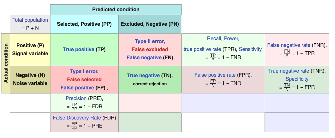
Precision and Recall
Recall = Power = Sensitivity = True positive rate
Precision = 1 - False discovery rate
 |
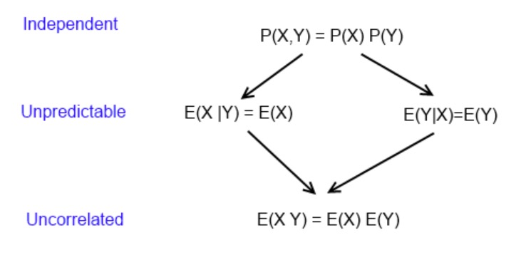
Independence, mean independence and uncorrelatedness
Statistical Independence \(\Longrightarrow\) Mean Independence \(\Longrightarrow\) Uncorrelatedness
\[ P(Y|X) = P(X) \Longrightarrow E(Y|X) = E(Y) \Longrightarrow cov(X,Y)=0 \]
The arrows can not be reversed.