fmristat
A general statistical analysis for fMRI data

The statistical analysis of the fMRI data was based on a linear model with correlated errors. The design matrix of the linear model was first convolved with a hemodynamic response function modeled as a difference of two gamma functions (Glover, 1999) timed to coincide with the acquisition of each slice. Drift was removed by adding polynomial covariates in the frame times to the design matrix. The correlation structure was modeled as an autoregressive process of degree 1 (Bullmore et al., 1996). At each voxel, the autocorrelation parameter was estimated from the least squares residuals using the Yule-Walker equations, after a bias correction for correlations induced by the linear model. The autocorrelation parameter was first regularized by spatial smoothing with a Gaussian filter, then used to `whiten' the data and the design matrix. The linear model was then re-estimated using least squares on the whitened data to produce estimates of effects and their standard errors.

In a second step, runs, sessions and subjects were combined using a mixed effects linear model for the effects (as data) with fixed effects standard deviations taken from the previous analysis. This was fitted using the the EM algorithm. A random effects analysis was performed by first estimating the the ratio of the random effects variance to the fixed effects variance, then regularzing this ratio by spatial smoothing with a Gaussian filter. The variance of the effect was then estimated by the smoothed ratio multiplied by the fixed effects variance to achieve higher degrees of freedom.

The resulting T statistic images were thresholded using the minimum given by a Bonferroni correction and random field theory (Worsley et al, 1996).

References

Bullmore, E.T., Brammer, M.J., Williams, S.C.R., Rabe-Hesketh, S., Janot, N., David, A.S., Mellers, J.D.C., Howard, R. and Sham, P. (1996). Statistical methods of estimation and inference for functional MR image analysis. Magnetic Resonance in Medicine, 35:261-277.

Glover, G.H. (1999). Deconvolution of impulse response in event-related BOLD fMRI. NeuroImage, 9:416-429.

Worsley, K.J., Marrett, S., Neelin, P., Vandal, A.C., Friston, K.J. and Evans, A.C. (1996). A unified statistical approach for determining significant signals in images of cerebral activation. Human Brain Mapping, 4:58-73.

The latest release of fmristat

Fmrilm and fmrilm_arp have been extended to estimate delays as well as effects with the addition of one more parameter, and fmridesign has been been extended to provide the necessary extra derivatives of the hrf. See the end of this document for instructions. (Note that the EXCLUDE parameter is no longer necessary for fmridesign and it must be ommitted.) The program can now estimate delays in seconds, shown below colouring the outer surface of the activated regions in top and cut-away front views. If you don't ask for delays, fmrilm and fmrilm_arp should be completely backwards compatible with previous versions.

[tstat>4.86 for a hot stimulus
coloured with the delay (seconds)]

Multistat has been updated to fit a random effects model by REML using the EM algorithm. This gives a better analysis than the previous version for combining subjects (the previous version was better at combining runs on the same subject, but this is usually not as important as combining subjects).

Tstat_threshold has been extended to find thresholds for F statistics as well as T statistics, and to find P-values for both if peak values are given instead. It also calculates P-values for the spatial extent of clusters of voxels above a threshold.

Locmax is a new function that finds local maxima of a minc file above a threshold.

Extract is a new function that extracts values from a minc file at specified voxels (in `register' format).

Example contains all the matlab commands for the example used here.

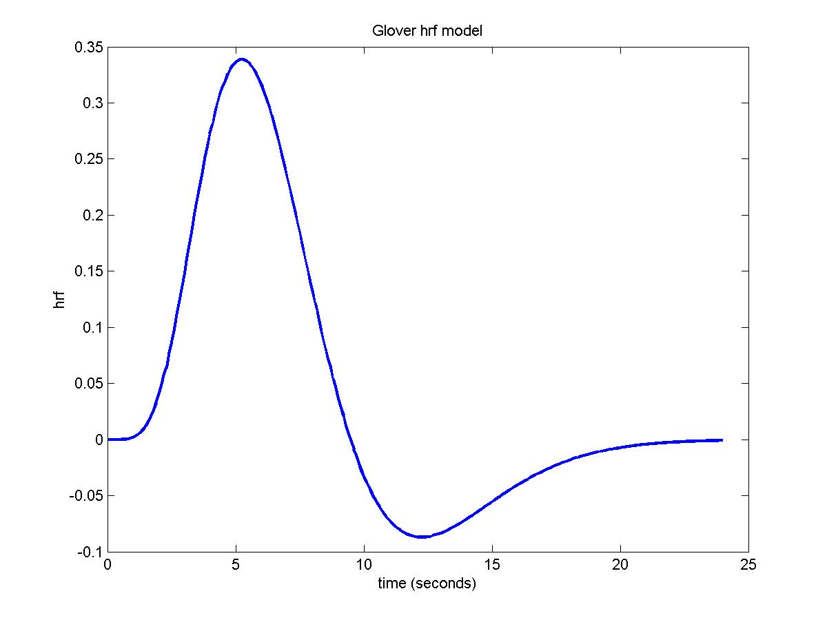
Plotting the hemodynamic response function (hrf) using fmridesign

The hrf is modeled as the difference of two gamma density functions (Glover, G.H. (1999). "Deconvolution of impulse response in event-related BOLD fMRI." NeuroImage, 9:416-429). The parameters of the hrf are specified by a row vector whose elements are:

1. PEAK1: time to the peak of the first gamma density;
2. FWHM1: approximate FWHM of the first gamma density;
3. PEAK2: time to the peak of the second gamma density;
4. FWHM2: approximate FWHM of the second gamma density;
5. DIP: coefficient of the second gamma density. The final hrf is: gamma1/max(gamma1)-DIP*gamma2/max(gamma2) scaled so that its total integral is 1.
6. NUM_DERIV: 0, 1 or 2 derivatives of h(t/c)/c with respect to log(c) at c=1, convolved with stimulus and added to X_cache. Used by FMRILM to estimate delays of the hrf.

If PEAK1=0 then there is no smoothing of that event type with the hrf. If PEAK1>0 but FWHM1=0 then the design is lagged by PEAK1. The default, chosen by Glover (1999) for an auditory stimulus, is:

hrf_parameters=[5.4 5.2 10.8 7.35 0.35 0] To look at the hemodynamic response function, try:
time=(0:240)/10; hrf0=fmridesign(time,0,[1 0],[],hrf_parameters); plot(time,hrf0,'LineWidth',2) xlabel('time (seconds)') ylabel('hrf') title('Glover hrf model')

Making the design matrices using fmridesign

Specifying all the frame times and slice times is now obligatory. For 120 scans, separated by 3 seconds, and 13 interleaved slices every 0.12 seconds use:

frametimes=(0:119)*3; slicetimes=[0.14 0.98 0.26 1.10 0.38 1.22 0.50 1.34 0.62 1.46 0.74 1.58 0.86]; The events are specified by a matrix of EVENTS, or directly by a stimulus design matrix S, or both. EVENTS is a matrix whose rows are events and whose columns are:

1. EVENTID - an integer from 1:(number of events) to identify event type;
2. EVENTIMES - start of event, synchronized with frame and slice times;
3. DURATION (optional - default is 0) - duration of event;
4. HEIGHT (optional - default is 1) - height of response for event.

For each event type, the response is a box function starting at the event times, with the specified durations and heights, convolved with the hemodynamic response function (see above). If the duration is zero, the response is the hemodynamic response function whose integral is the specified height - useful for ‘instantaneous’ stimuli such as visual stimuli. The response is then subsampled at the appropriate frame and slice times to create a design matrix for each slice, whose columns correspond to the event id number. EVENT_TIMES=[] will ignore event times and just use the stimulus design matrix S (see next).

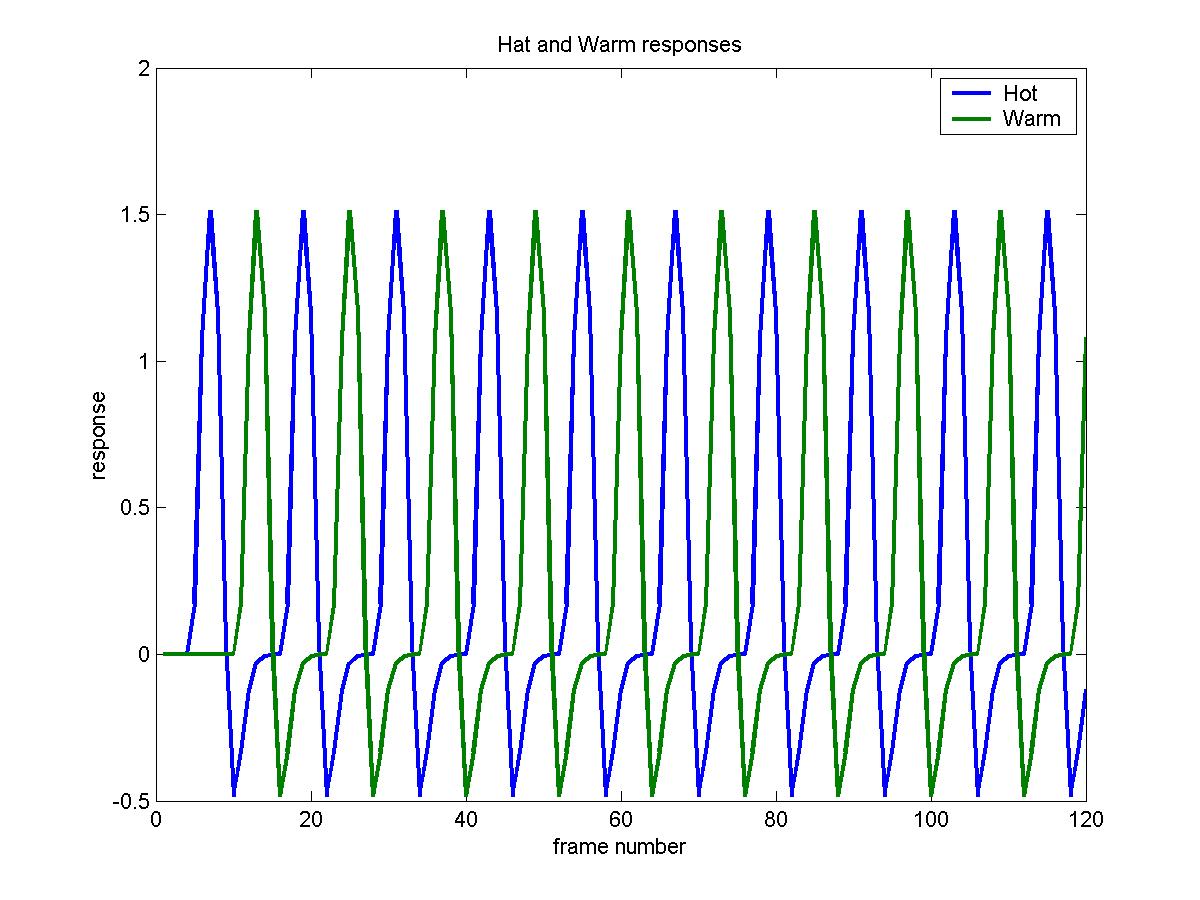
This is a sample run on Brian Ha's data, which was a block design of 3 scans rest, 3 scans hot stimulus, 3 scans rest, 3 scans warm stimulus, repeated 10 times (120 scans total). The hot event is identified by 1, and the warm event by 2. The events start at times 9,27,45,63... and each has a duration of 9s, with equal height:

eventid=kron(ones(10,1),[1; 2]); eventimes=(0:19)'*18+9; duration=ones(20,1)*9; height=ones(20,1); events=[eventid eventimes duration height] Events can also be supplied by a stimulus design matrix S (not recommended), whose rows are the frames, and columns are the event types. Events are created for each column, beginning at the frame time for each row of S, with a duration equal to the time to the next frame, and a height equal to the value of S for that row and column. Note that a constant term is not usually required, since it is removed by the polynomial trend terms provided N_POLY>=0. For the same experiment:
S=kron(ones(10,1),kron([0 0; 1 0; 0 0; 0 1],ones(3,1))); Either of these give the same cache of design matrices, X_CACHE, whose rows are frames, columns are all the regressor variables, with slices running slowest:
X_cache=fmridesign(frametimes,slicetimes,events,[],hrf_parameters); X_cache=fmridesign(frametimes,slicetimes, [] , S,hrf_parameters); or just
X_cache=fmridesign(frametimes,slicetimes,events); if you are using the default hrf parameters. To look at the two columns of the design matrix for the 5th slice (in columns 9 and 10 of X_CACHE):
plot(X_cache(:,9:10),'LineWidth',2) legend('Hot','Warm') xlabel('frame number') ylabel('response') title('Hat and Warm responses')

Analysing one run with fmrilm

First set up the contrasts. CONTRAST is a matrix whose rows are contrasts for the statistic images, with row length equal to the number regressor variables in X_CACHE plus N_POLY+1; the extra values allow you to set contrasts in the drift terms as well as the regressor variables. We wish to look for regions responding to the hot stimulus, the warm stimulus, and the difference hot-warm. Note that with N_POLY=3 (the default), the contrast matrix must be padded with 4 zeros:

contrast=[1 0 0 0 0 0; 0 1 0 0 0 0; 1 -1 0 0 0 0]; EXCLUDE is a list of frames that should be excluded from the analysis. This must be used with Siemens EPI scans to remove the first few frames, which do not represent steady-state images. Default is [1], but [1 2] is better:

exclude=[1 2]; WHICH_STATS is a logical matrix indicating output statistics by 1. Rows correspond to rows of CONTRAST, columns correspond to:

1: T statistic image, OUTPUT_FILE_BASE_tstat.mnc. The degrees of freedom is DF. Note that tstat=effect/sdeffect.
2: effect image, OUTPUT_FILE_BASE_effect.mnc.
3: standard deviation of the effect, OUTPUT_FILE_BASE_sdeffect.mnc.
4: F-statistic image, OUTPUT_FILE_BASE_Fstat.mnc, for testing all rows of CONTRAST simultaneously. The degrees of freedom are [DF, P].
5: the AR parameter, OUTPUT_FILE_BASE_rho.mnc.
6: the residuals from the model, OUTPUT_FILE_BASE_resid.mnc, only for the non-excluded frames (warning: uses lots of memory).
7: the whitened residuals from the model, OUTPUT_FILE_BASE_wresid.mnc, only for the non-excluded frames (warning: uses lots of memory).

If WHICH_STATS to a row vector of length 7, then it is used for all contrasts; if the number of columns is less than 7 it is padded with zeros. Default is 1.

To get t statistics, effects and their sd's, and the F statistic for testing for any effect of either hot or warm vs baseline:

which_stats=[1 1 1 1]; Input minc file for one session, and output base for each row of CONTRAST (hot for hot, wrm for warm, hmw for hot-warm):

input_file='/scratch/keith/brian_ha_19971124_1_093923_mri_MC.mnc'; output_file_base=['/scratch/keith/ha_093923_hot'; '/scratch/keith/ha_093923_wrm']; '/scratch/keith/ha_093923_hmw']; The big run:

[df1 p]=fmrilm(input_file, output_file_base, X_cache, contrast, exclude, which_stats); and the output gives the degrees of freedom of the T statistic images (df1=112) and the F statistic image (df1=112 , p=2). Note that p=2, not 3, because the third contrast is a linear combination of the first two.

F-tests should only be used when we are interested in any linear combination of the contrasts. For example, an F-test would be appropriate for detecting regions with high polynomial drift, since we would be interested in either a linear, quadratic or cubic trend, or any linear combination of these. To do this, use the contrast

contrast=[0 0 0 1 0 0; 0 0 0 0 1 0; 0 0 0 0 0 1] Another good use of the F-test is for detecting effects when the hemodynamic response is modeled by a set of basis functions (see below).

A linear effect of temperature

Instead of using just two values (hot=49^oC, and low=35^oC), suppose the temperature of the stimulus varied 'randomly' over the 20 blocks, taking 5 equally spaced values between 35 and 49:
temperature=[45.5 35.0 49.0 38.5 42.0 49.0 35.0 42.0 38.5 45.5 ... 38.5 49.0 35.0 45.5 42.0 45.5 38.5 42.0 35.0 49.0]'; To model a linear effect of temperature (see Figure (a) below), use one event type with height=1 and another with a height=temperature:
events=[zeros(20,1)+1 eventimes duration ones(20,1); zeros(20,1)+2 eventimes duration temperature] The following contrasts will estimate first the slope of the temperature effect (per ^oC), then the hot, warm and hot-warm effects exactly as before:
contrast=[0 1 0 0 0 0; 1 49 0 0 0 0; 1 35 0 0 0 0; 0 14 0 0 0 0];

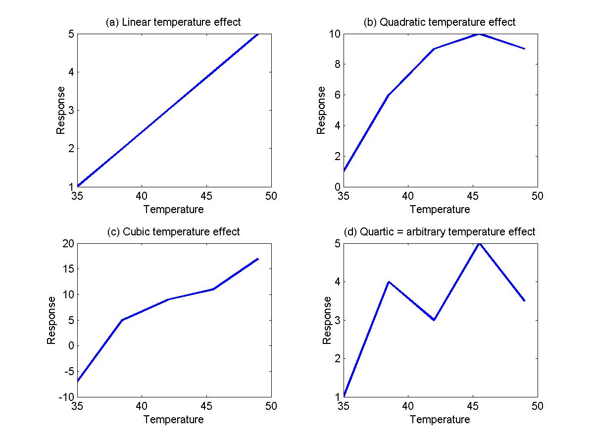
To model a quadratic effect of temperature (Figure b), add a third event type with a height equal to the temperature²:

events=[zeros(20,1)+1 eventimes duration ones(20,1); zeros(20,1)+2 eventimes duration temperature; zeros(20,1)+3 eventimes duration temperature^2] contrast=[0 0 1 0 0 0 0]; The contrast will test for a quadratic effect. Taking this further, we may wish to test for a cubic (Figure c), quartic (Figure d) or even a 'non-linear' effect of temperature, where the temperature effects are arbitrary. Note that the quartic model is identical to the arbitrary model because a quartic can be fitted exactly to any arbitrary 5 points. To model the arbitrary effect, simply assign a different event type from 1 to 5 for each of the 5 different temperature values: events=[floor((temperature-35)/3.5)+1 eventimes duration ones(20,1)] To look for any effect of the stimulus compared to baseline, use:
contrast=[1 0 0 0 0 0 0 0 0; 0 1 0 0 0 0 0 0 0; 0 0 1 0 0 0 0 0 0; 0 0 0 1 0 0 0 0 0; 0 0 0 0 1 0 0 0 0]; contrast=[eye(5) ones(5,4)]; which_stats=[0 0 0 1]; The resulting F statistic image will have 5 and 109 d.f.. To see if the changes in temperature have any effect, subtract the average from each row of the contrasts:
contrast=[.8 -.2 -.2 -.2 -.2 0 0 0 0; -.2 .8 -.2 -.2 -.2 0 0 0 0; -.2 -.2 .8 -.2 -.2 0 0 0 0; -.2 -.2 -.2 .8 -.2 0 0 0 0; -.2 -.2 -.2 -.2 .8 0 0 0 0]; contrast=[eye(5)-ones(5)/5 ones(5,4)]; which_stats=[0 0 0 1]; The resulting F statistic image will have 4 and 109 d.f.. To see if the changes in temperature have a linear effect, subtract the average from the 5 temperature values:
contrast=[-7.0 -3.5 0 3.5 7.0 0 0 0 0]; which_stats=[1 1 1]; This will produce a T statistic with 109 d.f.. How is this different from the previous linear effect? The effect is the same, but the standard deviation may be slightly different. The reason is that in this model, we are basing the standard deviation on errors about each temperature value; in the first analysis, it is based on errors about a linear model. As a result, the degrees of freedom is slightly different: 112 before, but 109 here.

Combining runs/sessions/subjects with multistat

Repeat previous analysis for three other sessions (note that the same X_CACHE is used for each):

input_file='/scratch/keith/brian_ha_19971124_1_100326_mri_MC.mnc'; output_file_base=['/scratch/keith/ha_100326_hot'; '/scratch/keith/ha_100326_wrm'; '/scratch/keith/ha_100326_hmw']; [df2 p]=fmrilm(input_file, output_file_base, X_cache, contrast, exclude, which_stats); input_file='/scratch/keith/brian_ha_19971124_1_101410_mri_MC.mnc'; output_file_base=['/scratch/keith/ha_101410_hot'; '/scratch/keith/ha_101410_wrm'; '/scratch/keith/ha_101410_hmw']; [df3 p]=fmrilm(input_file, output_file_base, X_cache, contrast, exclude, which_stats); input_file='/scratch/keith/brian_ha_19971124_1_102703_mri_MC.mnc'; output_file_base=['/scratch/keith/ha_102703_hot'; '/scratch/keith/ha_102703_wrm'; '/scratch/keith/ha_102703_hmw']; [df4 p]=fmrilm(input_file, output_file_base, X_cache, contrast, exclude, which_stats); Now we can average the different sessions as follows. NOTE THAT ALL FILES MUST HAVE EXACTLY THE SAME SHAPE (SLICES, COLUMNS, ROWS). If not, reshape them! This is done by again setting up design matrix and a contrast:

X=[1 1 1 1]'; contrast=[1]; which_stats=[1 1 1]; input_files_effect=['/scratch/keith/ha_093923_hmw_effect.mnc'; '/scratch/keith/ha_100326_hmw_effect.mnc'; '/scratch/keith/ha_101410_hmw_effect.mnc'; '/scratch/keith/ha_102703_hmw_effect.mnc']; input_files_sdeffect=['/scratch/keith/ha_093923_hmw_sdeffect.mnc'; '/scratch/keith/ha_100326_hmw_sdeffect.mnc'; '/scratch/keith/ha_101410_hmw_sdeffect.mnc'; '/scratch/keith/ha_102703_hmw_sdeffect.mnc']; output_file_base='/scratch/keith/ha_multi_hmw' For the final run, we need to specify the row vector of degrees of freedom of the input files, printed out by fmrilm.m:

input_files_df=[df1 df2 df3 df4] and their fwhm, in mm:

input_files_fwhm=6 These two parameters are only used to calculate the final degrees of freedom, and don't affect the images. Finally, for a fixed effects analysis (not recommended!) we set the last parameter to Inf (see later). The final run is:

df=multistat(input_files_effect,input_files_sdeffect,input_files_df, ... input_files_fwhm,X,contrast,output_file_base,which_stats,Inf) Note that the program prints and returns the final degrees of freedom of the tstat image, which is df=448 (see discussion on fixed and random effects).

For a more elaborate analysis, e.g. comparing the first two sessions with the next two, you can do it by:

X=[1 1 0 0; 0 0 1 1]'; contrast=[1 -1]; and the rest as above.

Fixed and random effects

In the above run, we did a fixed effect analysis, that is, the analysis is only valid for the particular group of 4 sessions on Brian Ha. It is not valid for an arbitrary session on Brian Ha, nor for the population of subjects in general. It may turn out that the underlying effects themselves vary from session to session, and from subject to subject. To take this extra source of variability into account, we should do a random effects analysis.

The ratio of the random effects standard error, divided by the fixed effects standard error, is outputed as ha_multi_sdratio.mnc. If there is no random effect, then sdratio should be roughly 1. If there is a random effect, sdratio will be greater than 1. To allow for the random effects, we multiply the sdeffect by sdratio, and divide the tstat by sdratio. The only problem is that sdratio is itself extremely noisy due to its low degrees of freedom, which results in a loss of sensitivity. One way around this is to assume that the underlying sdratio is fairly smooth, so it can be better estimated by smoothing sdratio. This will increase its degrees of freedom, thus increasing sensitivity. Note however that too much smoothing could introduce bias.

The amount of smoothing is controlled by the final parameter, fwhm_varatio. It is the fwhm in mm of the Gaussian filter used to smooth the ratio of the random effects variance divided by the fixed effects variance. 0 will do no smoothing, and give a purely random effects analysis. Inf will do complete smoothing to a global ratio of one, giving a purely fixed effects analysis (which we did above). The higher the fwhm_varatio, the higher the ultimate degrees of freedom of the tstat image (printed out before a pause), and the more sensitive the test. However too much smoothing will bias the results. The program prints and returns the df before doing any analysis; if it is too low, press control-c to cancel, and try increasing fwhm_varatio. The default is 15, and this is the recommended value. To invoke this, just run

df=multistat(input_files_effect,input_files_sdeffect,input_files_df, ... input_files_fwhm,X,contrast,output_file_base,which_stats,15) Note that the degrees of freedom of tstat is now reduced to df=112.

Thresholding the tstat image with tstat_threshold

Suppose we search /scratch/keith/ha_multi_tstat.mnc for local maxima inside a search region of 1000cc. The voxel volume is 2.34375*2.34375*7= 38.4521. There is 6mm smoothing. The degrees of freedom of is returned by multistat, is 112. The significance is the standard 0.05. The threshold to use is

tstat_threshold(1000000,38.4521,6,112,0.05) which gives 4.86. The resulting thresholded tstat is shown in the logo at the top of this page, rendered using IRIS Explorer. For the critical size of clusters above a threshold of say 3 use

tstat_threshold(1000000,38.4521,6,112,0.05,3) which gives peak_threshold=4.68 as above and extent_threshold=407 mm^3. This means that any cluster of neighbouring voxels above a threshold of 3 with a volume larger than 407 mm^3 is significant at P<0.05.

Reference:

Worsley, K.J., Marrett, S., Neelin, P., Vandal, A.C., Friston, K.J., and Evans, A.C. (1996). A Unified Statistical Approach for Determining Significant Signals in Images of Cerebral Activation. Human Brain Mapping, 4:58-73.

Locating peaks with locmax

To locate peaks, use
lm=locmax([output_file_base '_tstat.mnc'],4.68) which gives a list of local maxima above 4.68, sorted in descending order. The first column of LM is the values of the local maxima, and the next three are the x,y,z voxel coordinates in `register' format, i.e. starting at zero. To find P-values for these local maxima, replace the 0.05 by the list of peak values from the first column of LM:
pval=tstat_threshold(1000000,38.4521,6,448,lm(:,1))

Extracting values from a minc file using extract

You may want to look at the effects and their standard deviations at some of the local maxima just found, for example the peak with value 5.7629 in slice 5 with voxel coordinates [62 67 4]:
voxel=[62 67 4] effect=extract(voxel,output_file_base,'_effect.mnc') sdeffect=extract(voxel,output_file_base,'_sdeffect.mnc') which gives 5.0642 and 0.8788 respectively. Note that 5.0642/0.8788 = 5.7626, the value of the T statistic. A matrix of voxels can be given, and the corresponding vector of values will be extracted.

Estimating the delay

The last parameter of fmrilm is the REFERENCE_DELAY. There is one value for each event type, or if a single value is supplied, it is used for all event types. If the first element of REFERENCE_DELAY is >0 then delays are estimated as well as effects. We start with a reference hrf h(t) close to the true hrf, e.g. the Glover (1999) hrf used by FMRIDESIGN. The hrf for each variable is then modeled as h( t / c ) / c where c = DELAY / REFERENCE_DELAY, i.e. the time is re-scaled by c. The program then estimates contrasts in the c's (specified by CONTRAST; contrasts for the polynomial drift terms are ignored), their standard deviations, and T statistics for testing c=1 (no change). Output is DELAY = c * REFERENCE_DELAY in OUTPUT_FILE_BASE_delay.mnc, sd is in OUTPUT_FILE_BASE_sddelay.mnc, and t statistic in OUTPUT_FILE_BASE_tdelay.mnc. Note that REFERENCE_DELAY is only used to multiply c and its sd for output. If REFERENCE_DELAY is set equal to the first element of HRF_PARAMETERS (5.4 seconds by default) then DELAY is the estimated time to the first peak of the hrf (in seconds). To do the estimation, the stimuli must be convolved with first and second derivatives of h with respect to log(c) at c=1 and added to X_CACHE. FMRIDESIGN with the last element of HRF_PARAMETERS set to 2 does this for the Glover (1999) hrf. Note that F statistics are not yet available with this option. Default is 0, i.e. only effects are estimated.

Here is an example to estimate the delays of the hot and warm stimuli for the above data:

hrf_parameters2=[5.4 5.2 10.8 7.35 0.35 2] X_cache2=fmridesign(frametimes,slicetimes,events,[],hrf_parameters2); contrast=[1 0 0 0 0 0; 0 1 0 0 0 0] which_stats=[1 1 1 0] input_file='/scratch/keith/brian_ha_19971124_1_100326_mri_MC.mnc'; output_file_base=['/scratch/keith/ha_100326_delay_hot'; '/scratch/keith/ha_100326_delay_wrm'] n_poly=3; fwhm_rho=15; reference_delay=5.4; fmrilm(input_file, output_file_base, X_cache2, contrast, ... exclude, which_stats, fwhm_rho, n_poly, reference_delay); The result is 6 files for the hot stimulus, 3 for the effect:

/scratch/keith/ha_100326_delay_hot_tstat.mnc /scratch/keith/ha_100326_delay_hot_effect.mnc /scratch/keith/ha_100326_delay_hot_sdeffect.mnc and 3 for the delay (in seconds):

/scratch/keith/ha_100326_delay_hot_tdelay.mnc /scratch/keith/ha_100326_delay_hot_delay.mnc /scratch/keith/ha_100326_delay_hot_sddelay.mnc and 6 more for the warm stimulus. The best way of visualizing this is to use register like this: register /scratch/keith/ha_100326_delay_hot_tstat.mnc /scratch/keith/ha_100326_delay_hot_delay.mnc After synchronising the two images, you can then search the tstat image in the first window for regions of high signal e.g. >4, then read off the estimated delay at that location from the second window. A fancier rendering is shown at the top of this page.

Note that the tstat image is not quite the same as what you would get from fmrilm without asking for delays, i.e. with X_cache and REFERENCE_DELAY=0. The reason is that in order to calculate delays, fmrilm fits a model with convolutions of the stimulus with the derivative of the hrf added to the linear model.

You could now put delays and sddelays from separate runs/sessions/subjects through multistat as before.

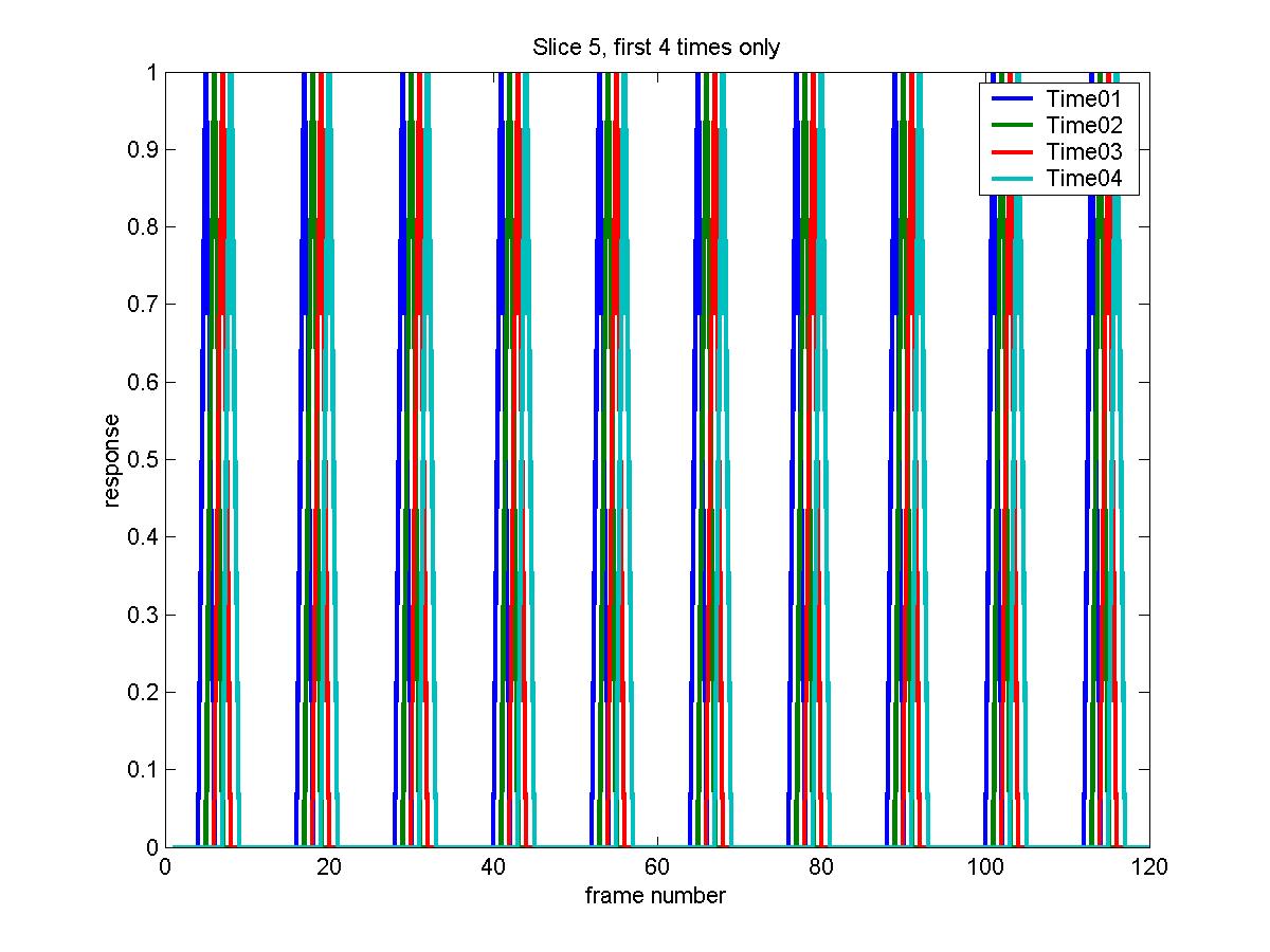
Estimating the time course of the response

We may be intersted in estimating the time course of the response. The easiest way to do this might be to average the responses beginning at the start of each `epoch' of the response, e.g. averaging the 12 scans starting at scans 1, 13, 25, ... 109. This does not remove drift, nor does it give you a standard error. A better, though more complex way, is to replace the block design of 2 blocks (9s hot, 9s warm) with say 12 blocks of 3s each covering the entire epoch, then estimate their effects with NO convolution by the hrf: eventid=kron(ones(10,1),(1:12)'); eventimes=frametimes'; duration=ones(120,1)*3; height=ones(120,1); events=[eventid eventimes duration height] X_cache=fmridesign(frametimes,slicetimes,events,[],zeros(1,6)); plot(X_cache(:,4*10+(1:4)),'LineWidth',2) legend('Time01','Time02','Time03','Time04') xlabel('frame number') ylabel('response') title('Slice 5, first 4 times only')

The advantage of this is that it is much more flexible; it can be applied to event related designs, with randomly timed events, even with events almost overlaping, and the duration of the `events' need not be equal to the TR. Moreover, the results from separate runs/sessions/subjects can be combined using multistat.

Now all the time course is covered by events, and the baseline has disappeared, so we must contrast each event with the average of all the other events, as follows:

contrast=[eye(12)-ones(12)/12 zeros(12,4)]; exclude=[1 2]; which_stats=[0 1 1 1]; input_file='/scratch/keith/brian_ha_19971124_1_100326_mri_MC.mnc'; output_file_base=['/scratch/keith/ha_100326_time01'; '/scratch/keith/ha_100326_time02'; '/scratch/keith/ha_100326_time03'; '/scratch/keith/ha_100326_time04'; '/scratch/keith/ha_100326_time05'; '/scratch/keith/ha_100326_time06'; '/scratch/keith/ha_100326_time07'; '/scratch/keith/ha_100326_time08'; '/scratch/keith/ha_100326_time09'; '/scratch/keith/ha_100326_time10'; '/scratch/keith/ha_100326_time11'; '/scratch/keith/ha_100326_time12']; fmrilm(input_file,output_file_base,X_cache,contrast,exclude,which_stats); We need 12 output files, but only the effect and its standard error. The F-statistic has been requested so we can find voxels with significant responses. Its critical threshold is:

tstat_threshold(1000000,38.4538,6,[11 103]) which gives 5.18. The local maxima above this are:

lm=locmax([output_file_base(1,:) '_fstat.mnc'],5.18) The extracted effects and their standard errors at the previous voxel=[62 67 4] are:

values=extract(voxel,output_file_base,'_effect.mnc') sd=extract(voxel,output_file_base,'_sdeffect.mnc') Plotting these out against time gives the estimated response, together with 1 sd error bars. Note that the times are offset by the slicetimes, so they are in seconds starting from the beginning of slice acquisition. On top of this we can add the modeled response by extracting the effects of the hot and warm stimuli, then multiplying these effects by the hrf convolved with the 9s blocks for hot and warm stimuli (also shown):

b_hot=extract(voxel,'/scratch/keith/ha_100326_hot','_effect.mnc') b_wrm=extract(voxel,'/scratch/keith/ha_100326_wrm','_effect.mnc') time=(1:360)/10; hrf_parameters=[5.4 5.2 10.8 7.35 0.35 0] hrf=fmridesign(time,0,[1 9 9 1],[],hrf_parameters); plot((0:12)*3+slicetimes(voxel(3)),values([1:12 1]),'k', ... [0:11; 0:11]*3+slicetimes(voxel(3)), [values+sd; values-sd],'g', ... time,[zeros(1,90) ones(1,90) zeros(1,180)],'r', ... time,[zeros(1,270) ones(1,90)],'b', ... time,hrf*b_hot+hrf([181:360 1:180])*b_wrm,'g'); legend('Estimated response','Modeled response'); text(10,0.5,'Hot') text(28,0.5,'Warm') xlabel('time (seconds) from start of epoch'); ylabel('fMRI response');

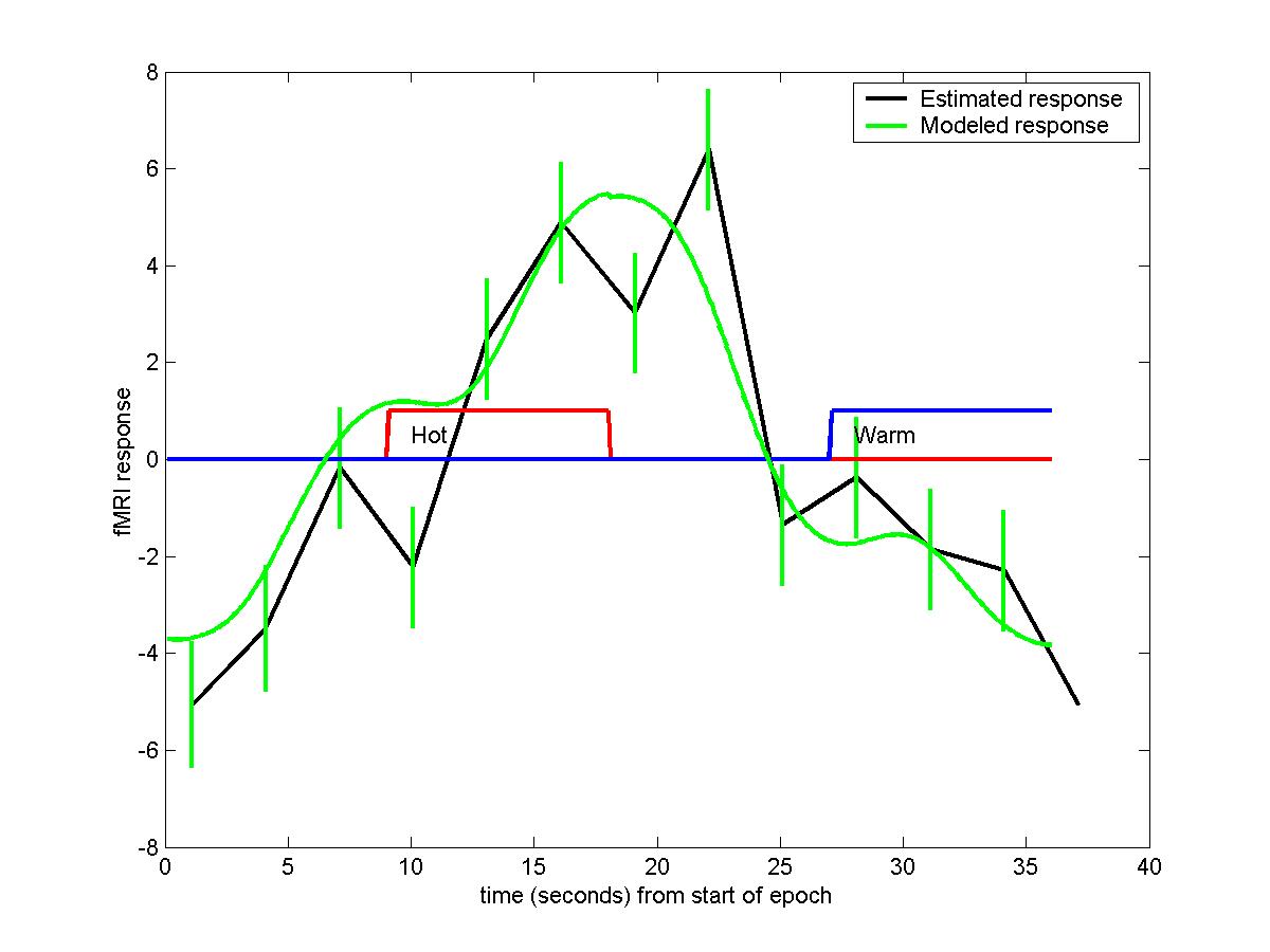
The modeled response and the fitted response are quite close. Note that the graph `wraps around' in time.

Estimating the hrf

We used the delay option to produce a 3D image of estimated delays of the hrf, but we may be interested in more details about the hrf. One way of doing this is to split up the hrf model into seperate components, similar to the way in which we split up the stimulus into seperate components to estimate the time course above. Rather than spliting up the hrf into blocks, we use a small number of overlapping gamma functions with different peak times. The idea is that we model the true hrf by a linear combination of these gamma functions (in fact the Glover hrf is a linear combination of 2 gamma funations, one for the main peak and one for the post-peak dip). In this example we use 4 gamma functions with peaks at 3s, 6s, 9s, and 12s, each with a width of 3s (the same as the TR):

hrf_peaks=[3:3:12] np=length(hrf_peaks) hrf_parameters=[ [hrf_peaks hrf_peaks]' 3*ones(2*np,1) zeros(2*np,4)] time=(0:240)/10; hrfs=fmridesign(time,0,[(1:np)' zeros(np,1)],[],hrf_parameters(1:np,:)); plot(time,hrfs,'LineWidth',2); xlabel('time (seconds)'); ylabel('hrf'); title('Hrf basis functions');

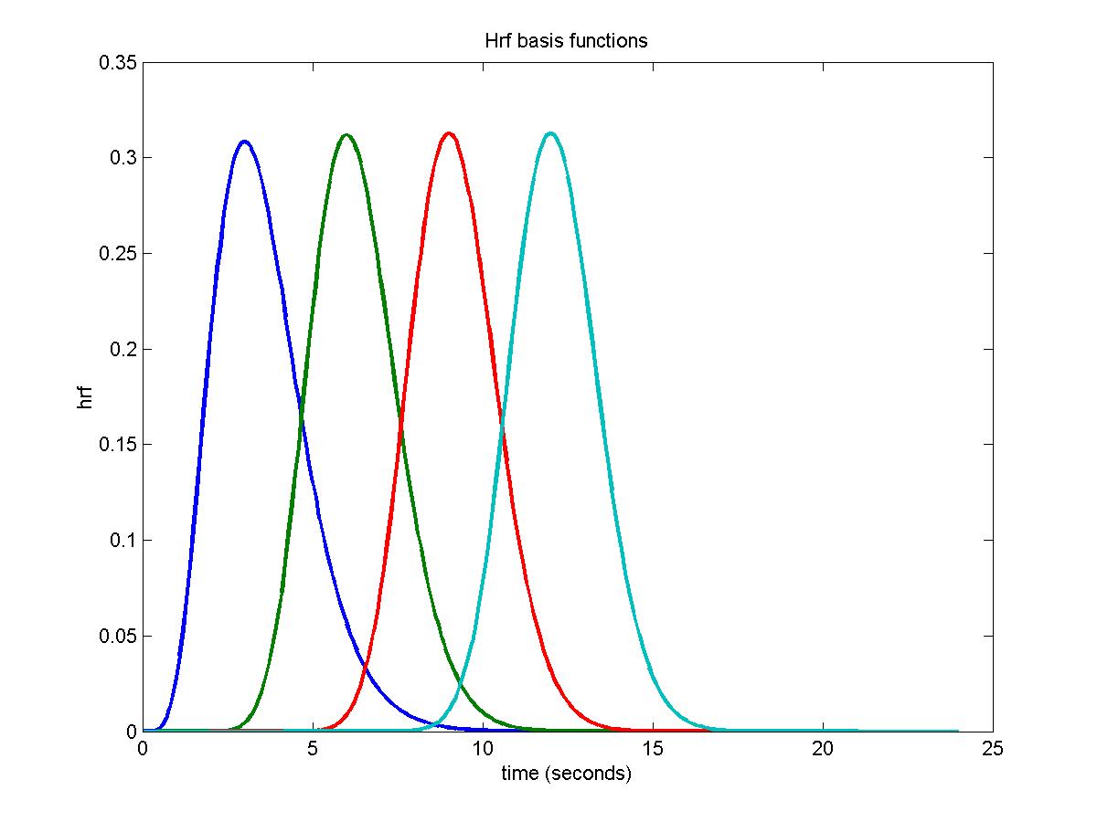
More basis functions will give more detail about the hrf, but because the resulting model is not very well conditioned (i.e. different linear combinations can fit more or less the same response model) then you get bizarre results, so you can't choose too many basis functions. I have found that separating the basis functions by the TR, and using a width equal to the TR, is about the best we can do. 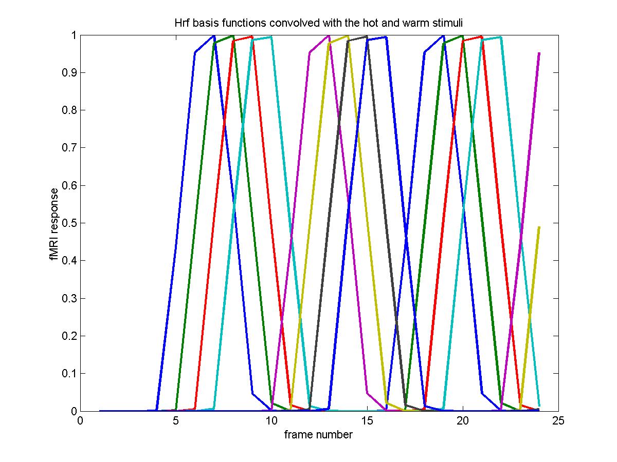In this example, we keep the original 9s hot and warm stimuli as before, but now we convolve them with the 4 different basis functions. This means that the hrf parameters are now an 8 x 6 matrix (4 rows for the hot, 4 rows for the warm stimuli) and the events are 4 repetitions of the original events, but with 4 new types for the hot and warm stimuli:

eventid=kron(ones(10,1),(1:2*np)'); eventimes=kron((0:19)'*18+9,ones(np,1)); duration=ones(20*np,1)*9; height=ones(20*np,1); events=[eventid eventimes duration height] X_cache=fmridesign(frametimes,slicetimes,events,[],hrf_parameters); plot(X_cache(1:24,1:2*np),'LineWidth',2) xlabel('frame number'); ylabel('fMRI response'); title('Hrf basis functions convolved with the hot and warm stimuli')

The CONTRAST compares each hrf to the average, as before, because the baseline has almost disappeared:

contrast=[eye(2*np)-ones(2*np)/2/np zeros(2*np,4)] which_stats=[0 1 1 1]; input_file='c:/keith/data/brian_ha_19971124_1_100326_mri_MC.mnc'; output_file_base=['c:/keith/data/ha_100326_hot1'; 'c:/keith/data/ha_100326_hot2'; 'c:/keith/data/ha_100326_hot3'; 'c:/keith/data/ha_100326_hot4'; 'c:/keith/data/ha_100326_wrm1'; 'c:/keith/data/ha_100326_wrm2'; 'c:/keith/data/ha_100326_wrm3'; 'c:/keith/data/ha_100326_wrm4']; fmrilm(input_file, output_file_base, X_cache,contrast,exclude, which_stats); Once again we pick a voxel with a big F statistic, find the coefficients of the 4 basis functions for the hot and warm stimuli, multiply them by the hrf basis functions, add, and plot out against time, together with the Glover hrf's for comparison:

tstat_threshold(1000000,38.4538,6,[7 106]) lm=locmax([output_file_base(1,:) '_fstat.mnc'],6.5642) voxel=[62 65 4] coefs=extract(voxel,output_file_base,'_effect.mnc') sdcoefs=extract(voxel,output_file_base,'_sdeffect.mnc') b_hot=extract(voxel,'c:/keith/data/ha_100326_hot','_effect.mnc') b_wrm=extract(voxel,'c:/keith/data/ha_100326_wrm','_effect.mnc') hrf0=fmridesign(time); plot(time, [hrfs*coefs(1:np)' hrf0*b_hot hrfs*coefs((1:np)+np)' hrf0*b_wrm], ... 'LineWidth',2); legend('Hot estimated','Hot model','Warm estimated','Warm model'); xlabel('time (seconds)'); ylabel('hrf'); title('Estimated hrfs for the hot and warm stimuli, together with the Glover hrfs')

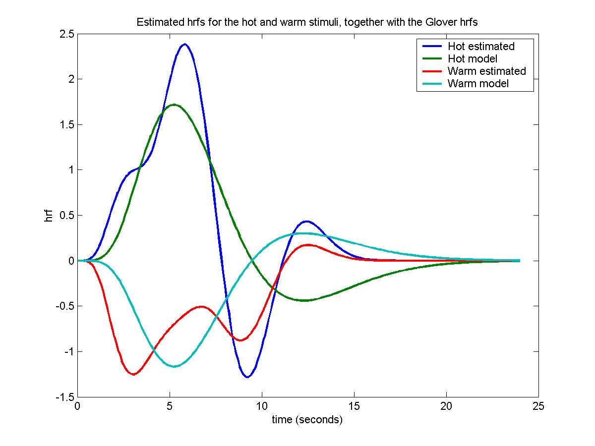
The Glover hrfs seem to be quite close to the estimated hrfs, but the standard deviations of the coefficients are really big, almost the same size as the coefficients themselves, so that the estimated hrfs are very inaccurate. In fact, moving to neighbouring pixels in the same slice produces dramatically different estimated hrfs.

fmristatA general statistical analysis for fMRI data

Summary of method